from pathlib import Path
import numpy as np
from matplotlib import pyplot as plt
import spikeinterface.core as si
import spikeinterface.preprocessing as spre
from spikeinterface.core.generate import (
    generate_unit_locations,
    generate_templates,
    generate_ground_truth_recording,
    default_unit_params_range,
)
from spikeinterface.curation import MergeUnitsSorting
from spikeinterface import aggregate_units
from probeinterface import generate_multi_columns_probe
from probeinterface.plotting import plot_probe
import UnitMatchPy as um
import UnitMatchPy.default_params as default_paramsI recently consulted on a project where chronic recordings from mice were made with implanted electrodes. This presents challenges: processing multi-day recordings in one go is highly inefficient or impossible due to memory limitations. While dividing data into chunks enables parallel processing, it creates a new problem: the units identified in different recording segments do not follow the same order (e.g. unit 1 in recording 1 is likely not the same as unit 1 in recording 2). Thus, the units must somehow be matched across recordings based on physiological features.
While searching for solutions to this problem, I came across UnitMatch - an algorithm that uses a naive Bayes classifier to match units based on their average spike waveforms (more on that later). The algorithm was published in Nature Methods and there is a Matlab and a Python toolbox available. Unfortunately, I found that the project lacks documentation and existing tutorial notebooks contained errors or were incomplete (due to missing data).
To test and verify the functionalities of UnitMatch, I created this notebook where I simulate multiple electrophysiological recordings with SpikeInterface and identify matching units across recordings. I hope prospective UnitMatch users will find it useful. Feel free to play around with the parameters of the simulation and UnitMatch to see how it affects the results. To follow along with the examples, you’ll have to install the following packages (I recommend using a new virtual environment).
pip install numpy matplotlib spikeinterface UnitMatchPySimulating Data with SpikeInterface
This section simulates multiple electrophysiological recordings and their corresponding spike sorting results. The basic idea is that we generate a template waveform for each unit and then simulate the recordings from these template waveforms. The waveform parameters will be slightly varied across recordings to simulate the variability expected in chronic recordings (e.g. due to movement of the electrodes). First, we need to define the parameters for the simulated data.
seed = 100  # set seed for reproducibility
n_recordings = 3  # number of recordings
n_units = 10  # number of units
n_columns = 2  # number of electrode columns
n_contacts = 6  # number of channels per column
To simulate recordings, we generate a probe and unit locations along it. The probe and unit locations will be the same for all recording segments.
probe = generate_multi_columns_probe(
    num_columns=n_columns, num_contact_per_column=n_contacts
)
probe.set_device_channel_indices(range(probe.get_contact_count()))
channel_locations = probe.contact_positions
unit_locations = generate_unit_locations(
    num_units=n_units, channel_locations=channel_locations, seed=seed
)
fig, ax = plt.subplots()
plot_probe(probe, ax=ax)
ax.scatter(unit_locations[:, 0], unit_locations[:, 1], label="Units")
ax.legend()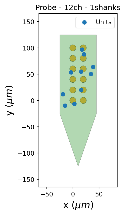
Next, we generate a dictionary that contains the parameters for the template waveform of every unit. SpikeInterface provides the dictionary default_unit_params_range that contains the default range of parameter values for simulating units (e.g. amplitude or spatial decay). For each unit, we’ll sample a value from that range. The result is the dictionary unit_params that stores arrays where each element is the parameter for one unit.
rng = np.random.default_rng(seed)
unit_params = {}
for key, (low, high) in default_unit_params_range.items():
    unit_params[key] = rng.uniform(low, high, size=n_units)
unit_params
{'alpha': array([433.9926522 , 338.62161079, 215.54529668, 117.18062828,
489.46175804, 338.58868163, 416.10526577, 464.13575252,
375.26177904, 175.99658936]),
'depolarization_ms': array([0.13907395, 0.104237 , 0.12146366, 0.11905182, 0.11999561,
0.11676241, 0.13978886, 0.1150973 , 0.12855113, 0.11470809]),
'repolarization_ms': array([0.79930235, 0.79358658, 0.61807041, 0.59657758, 0.7586542 ,
0.73979747, 0.70742919, 0.62255536, 0.61692954, 0.53949452]),
'recovery_ms': array([1.31274874, 1.04120069, 1.13728649, 1.32805851, 1.00733802,
1.41726609, 1.03619954, 1.26206041, 1.27327526, 1.11362348]),
'positive_amplitude': array([0.24339673, 0.15114458, 0.17570612, 0.23010754, 0.19854294,
0.15770836, 0.11444086, 0.24337084, 0.18843507, 0.18732443]),
'smooth_ms': array([0.05388581, 0.03595496, 0.05240195, 0.0525267 , 0.05323953,
0.03739796, 0.05838476, 0.03280083, 0.0429946 , 0.03427422]),
'spatial_decay': array([34.96057387, 30.03148015, 29.32616207, 21.47386745, 28.84192769,
24.47022155, 26.05951453, 27.88696017, 34.13261297, 35.72726278]),
'propagation_speed': array([285.68360953, 317.01298515, 301.022312 , 317.11452607,
283.03320714, 339.84195609, 316.27920104, 269.17973465,
307.51585252, 324.94028809]),
'b': array([0.8019328 , 0.49395841, 0.35048142, 0.65442167, 0.75691121,
0.55651163, 0.26614706, 0.65286473, 0.78431686, 0.92351301]),
'c': array([0.99500395, 0.43145132, 0.8250356 , 0.72058249, 0.97564282,
0.55789109, 0.87457736, 0.5536417 , 0.35942747, 0.96434435]),
'x_angle': array([8.92445114e-01, 9.75961624e-01, 1.87809180e-01, 1.43342828e-03,
1.07303982e+00, 8.50411327e-01, 2.28247368e+00, 4.60233512e-02,
2.80095771e+00, 2.56516667e+00]),
'y_angle': array([2.85774694, 2.41109034, 2.06560572, 2.39953077, 2.76379207,
2.68240018, 0.8497379 , 2.99180754, 3.11848977, 2.17921963]),
'z_angle': array([1.92613828, 1.92716042, 2.1546994 , 2.84738271, 0.97173317,
1.25863705, 0.99223389, 2.26800388, 0.10700536, 1.26789758])}For each recording, we’ll add a bit of random noise to these parameters to simulate the variability that is expected across recordings (feel free to play around with the variability parameter to see how it affects the matching results). The varied_params are passed to the generate_templates function and the generated waveforms are stored in a list of templates.
variability = 0.02
templates = []
for i in range(n_recordings):
    varied_params = {}
    for key in unit_params.keys():  # vary unit parameters
        variation = rng.normal(0, variability * unit_params[key])
        varied_params[key] = unit_params[key] + variation

    templates.append(
        generate_templates(
            channel_locations=channel_locations,
            units_locations=unit_locations,
            sampling_frequency=25000,
            unit_params=varied_params,
            ms_before=1.0,
            ms_after=3.0,
            seed=seed,
        )
    )
Let’s plot the same unit across multiple recordings. Despite slight variability, the waveforms are similar enough to enable clear matching.
fig, ax = plt.subplots(1, 3, figsize=(9, 3), sharex=True, sharey=True)
for i in range(3):
    ax[i].plot(templates[i][0, :, :])
    ax[i].set(title=f"Recording {i+1}")
ax[0].set(ylabel=r"Voltage [$\mu$V]")
ax[1].set(xlabel="Time [samples]")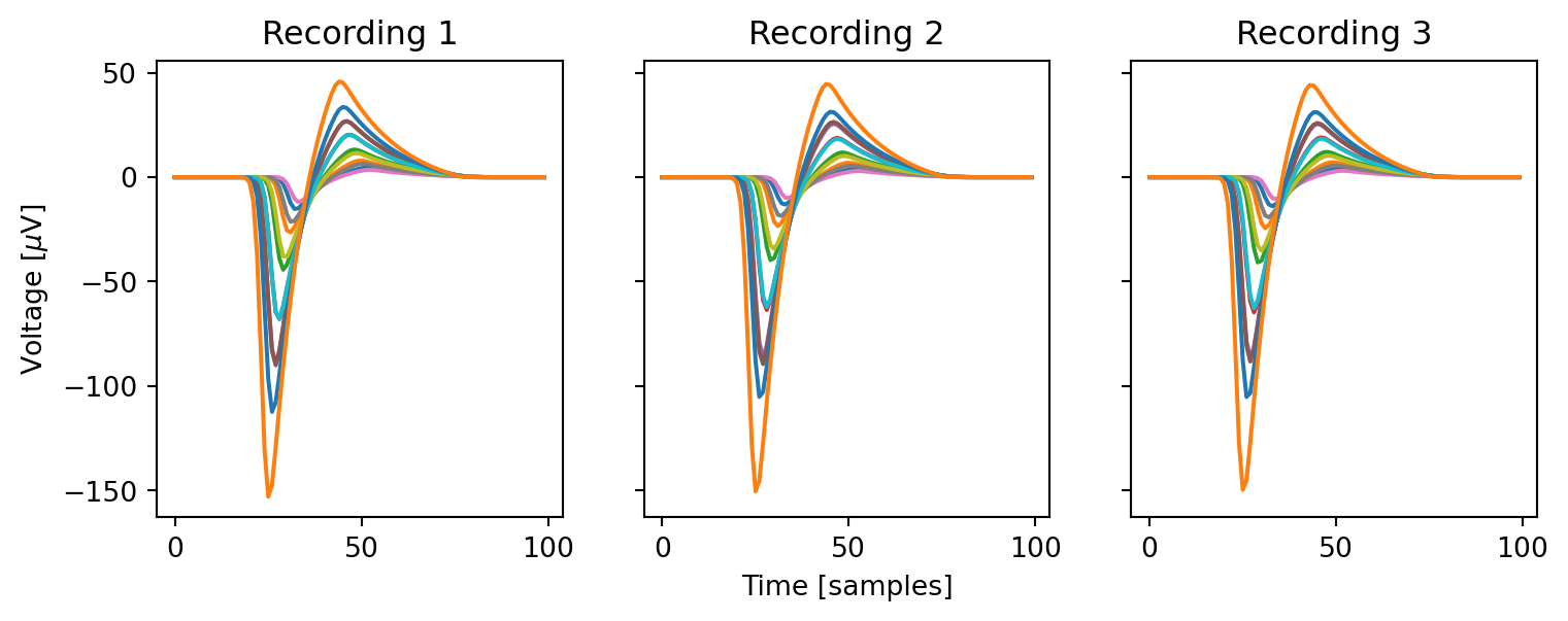
Finally, we use the generate_ground_truth_recording function to generate a list of recordings and sortings from the previously created templates.
recordings, sortings = [], []
for i, template in enumerate(templates):
    recording, sorting = generate_ground_truth_recording(
        num_units=n_units, probe=probe, templates=template, seed=seed
    )
    recordings.append(recording)
    sortings.append(sorting)
recordings, sortings
([GroundTruthRecording (InjectTemplatesRecording): 12 channels - 25.0kHz - 1 segments
250,000 samples - 10.00s - float32 dtype - 11.44 MiB,
GroundTruthRecording (InjectTemplatesRecording): 12 channels - 25.0kHz - 1 segments
250,000 samples - 10.00s - float32 dtype - 11.44 MiB,
GroundTruthRecording (InjectTemplatesRecording): 12 channels - 25.0kHz - 1 segments
250,000 samples - 10.00s - float32 dtype - 11.44 MiB],
[GroundTruthSorting (NumpySorting): 10 units - 1 segments - 25.0kHz,
GroundTruthSorting (NumpySorting): 10 units - 1 segments - 25.0kHz,
GroundTruthSorting (NumpySorting): 10 units - 1 segments - 25.0kHz])Preprocessing and Curation
Since UnitMatch uses average unit waveforms, we must ensure they’re clearly visible across multiple recording sites. To achieve this, we’ll preprocess the recordings and select units based on quality criteria. For the simulated data, I am only applying a bandpass filter, but real data may require additional steps such as correcting the small sampling delay across channels that some systems (e.g. Neuropixels) introduce or applying motion correction (note that this only corrects motion within, not across, recordings).
for i, recording in enumerate(recordings):
    recording = spre.bandpass_filter(recording, freq_min=300, freq_max=3000)
    # recording = spre.phase_shift(recording)
    # recording = spre.correct_motion(recording, preset="nonrigid_fast_and_accurate")
    recordings[i] = recording
recordings
[GroundTruthRecording (BandpassFilterRecording): 12 channels - 25.0kHz - 1 segments
250,000 samples - 10.00s - float32 dtype - 11.44 MiB,
GroundTruthRecording (BandpassFilterRecording): 12 channels - 25.0kHz - 1 segments
250,000 samples - 10.00s - float32 dtype - 11.44 MiB,
GroundTruthRecording (BandpassFilterRecording): 12 channels - 25.0kHz - 1 segments
250,000 samples - 10.00s - float32 dtype - 11.44 MiB]Next, we calculate waveform templates from the recordings. To do this, we create an analyzer object by pairing each recording and sorting and compute “extensions” that are added to the analyzer. These extensions partly depend on each other — for example, computing the "templates" extension requires the "random_spikes" extension to be computed. Important: UnitMatch expects the waveform to be symmetric around the spike, so when you use different values for ms_before and ms_after, you’ll have to set the respective parameter in UnitMatch.
analyzers = []
for sorting, recording in zip(sortings, recordings):
    analyzer = si.create_sorting_analyzer(sorting, recording, sparse=False)
    analyzer.compute("random_spikes", method="uniform", max_spikes_per_unit=500)
    analyzer.compute("templates", ms_before=2, ms_after=2)
    analyzers.append(analyzer)
analyzers
[SortingAnalyzer: 12 channels - 10 units - 1 segments - memory - has recording
Loaded 2 extensions: random_spikes, templates,
SortingAnalyzer: 12 channels - 10 units - 1 segments - memory - has recording
Loaded 2 extensions: random_spikes, templates,
SortingAnalyzer: 12 channels - 10 units - 1 segments - memory - has recording
Loaded 2 extensions: random_spikes, templates]Let’s look at two of the extracted templates. In the figure below, we can clearly see one unit that has a large amplitude and is visible across all channels, and another one with a weak and noisy signal.
templates = analyzers[0].get_extension("templates").get_data()
fig, ax = plt.subplots(1, 2, figsize=(6, 3), sharex=True, sharey=False)
for i, uid in enumerate([0, 3]):
    ax[i].plot(templates[uid, :, :])
    ax[i].set(title=f"Unit {uid+1}")
ax[0].set(ylabel=r"Voltage [$\mu$V]")
ax[1].set(xlabel="Time [samples]")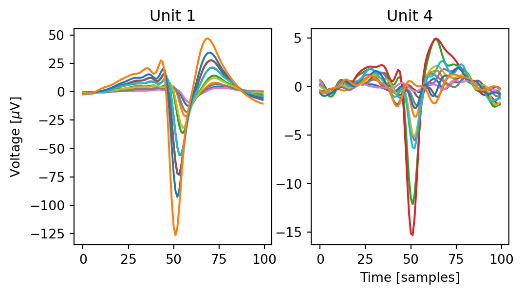
To remove the latter unit and others like it, we compute "quality_metrics" and select only those units that meet our quality criteria. Since most quality criteria (like ISI violations) don’t apply to simulated data, we’ll use only signal-to-noise ratio for unit selection. However, for real data that is probably insufficient — I recommend this notebook for an overview and discussion of different quality criteria.
min_snr = 10
for i, analyzer in enumerate(analyzers):
    analyzer.compute("noise_levels")  # required to compute SNR
    analyzer.compute("quality_metrics", metric_names=["snr"])
    metrics = analyzer.get_extension("quality_metrics").get_data()
    keep_mask = metrics.snr > min_snr
    keep_unit_ids = sorting.unit_ids[keep_mask]
    print(f"Keeping {len(keep_unit_ids)} out of {len(sorting.unit_ids)} units")
    sortings[i] = sortings[i].select_units(keep_unit_ids)

fig, ax = plt.subplots()
ax.hist(metrics.snr)
ax.axvline(x=min_snr, ymin=0, ymax=1, color="red", linestyle="--")
ax.set(ylabel="Number of Units", xlabel="SNR", title="SNR Distribution in Recording 3")
Keeping 9 out of 10 unitsKeeping 8 out of 10 unitsKeeping 8 out of 10 units[Text(0, 0.5, 'Number of Units'),
Text(0.5, 0, 'SNR'),
Text(0.5, 1.0, 'SNR Distribution in Recording 3')]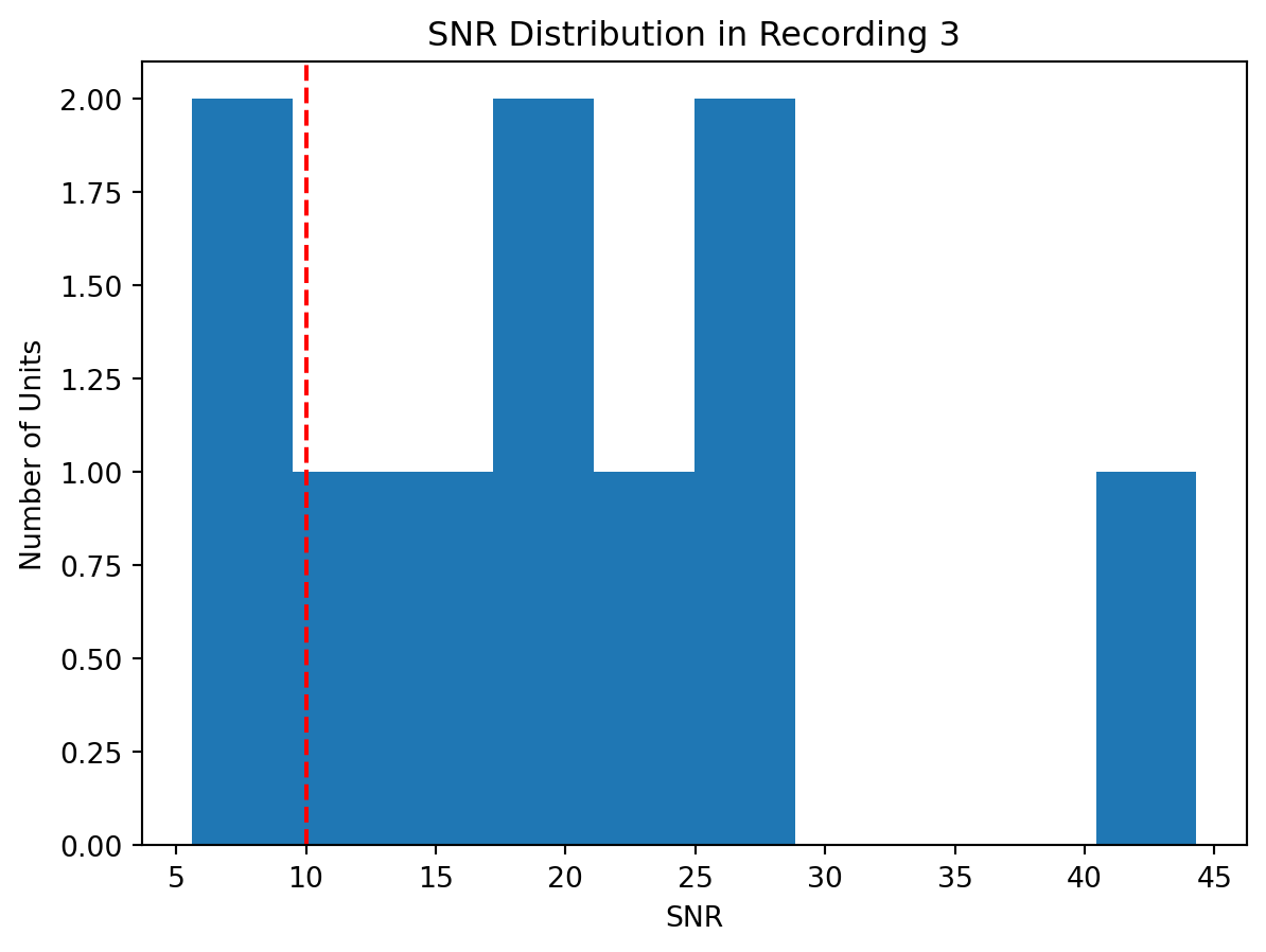
Preparing the Data for UnitMatch
Next, we convert SpikeInterface data to UnitMatch’s expected format. First, we create a directory "UMInputData" with a subdirectory for each session and a "RawWaveforms" subdirectory in each session’s directory.
UM_input_dir = Path("UMInputData").absolute()
for i in range(len(recordings)):
    session_dir = UM_input_dir / f"Session{i+1}"
    (session_dir / "RawWaveforms").mkdir(parents=True, exist_ok=True)
!tree UMInputData
UMInputData ├── Session1 │ ├── RawWaveforms │ │ ├── Unit0_RawSpikes.npy │ │ ├── Unit1_RawSpikes.npy │ │ ├── Unit2_RawSpikes.npy │ │ ├── Unit3_RawSpikes.npy │ │ ├── Unit4_RawSpikes.npy │ │ ├── Unit5_RawSpikes.npy │ │ ├── Unit6_RawSpikes.npy │ │ └── Unit7_RawSpikes.npy │ ├── channel_positions.npy │ └── cluster_group.tsv ├── Session2 │ ├── RawWaveforms │ │ ├── Unit0_RawSpikes.npy │ │ ├── Unit1_RawSpikes.npy │ │ ├── Unit2_RawSpikes.npy │ │ ├── Unit3_RawSpikes.npy │ │ ├── Unit4_RawSpikes.npy │ │ ├── Unit5_RawSpikes.npy │ │ ├── Unit6_RawSpikes.npy │ │ └── Unit7_RawSpikes.npy │ ├── channel_positions.npy │ └── cluster_group.tsv └── Session3 ├── RawWaveforms │ ├── Unit0_RawSpikes.npy │ ├── Unit1_RawSpikes.npy │ ├── Unit2_RawSpikes.npy │ ├── Unit3_RawSpikes.npy │ ├── Unit4_RawSpikes.npy │ ├── Unit5_RawSpikes.npy │ ├── Unit6_RawSpikes.npy │ └── Unit7_RawSpikes.npy ├── channel_positions.npy └── cluster_group.tsv 7 directories, 30 files
Next, we need to extract the channel locations from every recording and store them in the session directory as "channel_positions.npy".
for i, (recording, sorting) in enumerate(zip(recordings, sortings)):
    channel_locations = recording.get_channel_locations()
    np.save(UM_input_dir / f"Session{i+1}" / "channel_positions.npy", channel_locations)
Next, we create a table for each recording storing the original cluster ID of each unit (as assigned by the spike sorter) and the “group” to which it belongs. For the simulated data, all units are labeled "good" but for actual recordings you may want to label some as "mua" (multi-unit activity). The table is stored in the session directory as "cluster_group.tsv".
for i, (recording, sorting) in enumerate(zip(recordings, sortings)):
    n_units = sorting.get_num_units()
    cluster_group = np.stack((range(n_units), ["good" for i in range(n_units)]), axis=1)
    cluster_group = np.vstack((np.array(("cluster_id", "group")), cluster_group))
    np.savetxt(
        UM_input_dir / f"Session{i+1}" / "cluster_group.tsv", cluster_group, fmt="%s", delimiter="\t"
    )
cluster_group
array([['cluster_id', 'group'],
['0', 'good'],
['1', 'good'],
['2', 'good'],
['3', 'good'],
['4', 'good'],
['5', 'good'],
['6', 'good'],
['7', 'good']], dtype='<U21')Now comes the critical part: each recording and sorting has to be divided into two parts. UnitMatch calibrates the matching threshold by comparing units between the first and second half of each recording. We’ll split every recording and sorting into two and append the pieces to lists. From this, we obtain the lists of lists split_recordings and split_sortings where each element is a list with the first and second half of a given sorting/recording.
split_recordings, split_sortings = [], []
for sorting, recording in zip(sortings, recordings):
    n = recording.get_num_samples()
    split_sortings.append(  # split sortings
        [
            sorting.frame_slice(start_frame=0, end_frame=n // 2),  # 1st half
            sorting.frame_slice(start_frame=n // 2, end_frame=n),  # 2nd half
        ]
    )
    split_recordings.append(  # split recordings
        [
            recording.frame_slice(start_frame=0, end_frame=n // 2),  # 1st half
            recording.frame_slice(start_frame=n // 2, end_frame=n),  # 2nd half
        ]
    )
split_sortings
[[GroundTruthSorting (FrameSliceSorting): 9 units - 1 segments - 25.0kHz,
GroundTruthSorting (FrameSliceSorting): 9 units - 1 segments - 25.0kHz],
[GroundTruthSorting (FrameSliceSorting): 8 units - 1 segments - 25.0kHz,
GroundTruthSorting (FrameSliceSorting): 8 units - 1 segments - 25.0kHz],
[GroundTruthSorting (FrameSliceSorting): 8 units - 1 segments - 25.0kHz,
GroundTruthSorting (FrameSliceSorting): 8 units - 1 segments - 25.0kHz]]For the half recordings and sortings, we’ll have to create new analyzers. The analyzers are stored in another list of lists called split_analyzers.
split_analyzers = []
for recording, sorting in zip(split_recordings, split_sortings):
    split_analyzers.append(
        [
            si.create_sorting_analyzer(sorting[0], recording[0], sparse=False),
            si.create_sorting_analyzer(sorting[1], recording[1], sparse=False),
        ]
    )
split_analyzers
[[SortingAnalyzer: 12 channels - 9 units - 1 segments - memory - has recording
Loaded 0 extensions,
SortingAnalyzer: 12 channels - 9 units - 1 segments - memory - has recording
Loaded 0 extensions],
[SortingAnalyzer: 12 channels - 8 units - 1 segments - memory - has recording
Loaded 0 extensions,
SortingAnalyzer: 12 channels - 8 units - 1 segments - memory - has recording
Loaded 0 extensions],
[SortingAnalyzer: 12 channels - 8 units - 1 segments - memory - has recording
Loaded 0 extensions,
SortingAnalyzer: 12 channels - 8 units - 1 segments - memory - has recording
Loaded 0 extensions]]We extract template waveforms from each half recording using the split_analyzers. We’ll compute the "templates" extension on every analyzer, stack the waveforms of the first and second half into a single array and append it to a list called all_waveforms. Each element in all_waveforms is a 4-dimensional numpy array where the dimensions represent units, samples, channels, and halves.
all_waveforms = []
for analyzer in split_analyzers:
    # waveforms for 1st half
    analyzer[0].compute("random_spikes", method="uniform", max_spikes_per_unit=500)
    analyzer[0].compute("templates", ms_before=2, ms_after=2, n_jobs=0.8)
    # waveforms for 2nd half
    analyzer[1].compute("random_spikes", method="uniform", max_spikes_per_unit=500)
    analyzer[1].compute("templates", ms_before=2, ms_after=2, n_jobs=0.8)
    # get waveform arrays and append them to list
    all_waveforms.append(
        np.stack(
            (
                analyzer[0].get_extension("templates").get_data(),
                analyzer[1].get_extension("templates").get_data(),
            ),
            axis=-1,
        )
    )
all_waveforms[0].shape
(9, 100, 12, 2)Finally, we can save the waveforms to the session folders. For this, we’ll use the save_avg_waveforms function from UnitMatchPy. This function takes as arguments the average waveforms for a given session, the path to the session directory, as well as the previously created cluster_group table (so we’ll have to load that again). The save_avg_waveforms function will store one numpy array for every unit in the RawWaveforms subdirectory within the session directory.
for i in range(len(all_waveforms)):
    session_dir = UM_input_dir / f"Session{i+1}"
    cluster_group = np.loadtxt(  # load table with good units
        session_dir / "cluster_group.tsv", delimiter="\t", dtype=str
    )
    um.extract_raw_data.save_avg_waveforms(
        all_waveforms[i],
        session_dir,
        cluster_group,
    )
!tree UMInputData/Session1
Saved 10 units to RawWaveforms directory, saving all units Saved 9 units to RawWaveforms directory, saving all units Saved 9 units to RawWaveforms directory, saving all units UMInputData/Session1 ├── RawWaveforms │ ├── Unit0_RawSpikes.npy │ ├── Unit1_RawSpikes.npy │ ├── Unit2_RawSpikes.npy │ ├── Unit3_RawSpikes.npy │ ├── Unit4_RawSpikes.npy │ ├── Unit5_RawSpikes.npy │ ├── Unit6_RawSpikes.npy │ ├── Unit7_RawSpikes.npy │ └── Unit8_RawSpikes.npy ├── channel_positions.npy └── cluster_group.tsv 2 directories, 11 files
Extracting Waveform Properties and Matching Units
With the data stored, we’re ready to run UnitMatch. The first step is to load the default parameters. The param dictionary contains the parameters for the UnitMatch algorithm and will be read and modified by multiple functions in the pipeline.
param = default_params.get_default_param()
param.keys()
dict_keys(['spike_width', 'waveidx', 'channel_radius', 'peak_loc', 'max_dist', 'neighbour_dist', 'stepsz', 'smooth_prob', 'min_angle_dist', 'min_new_shank_distance', 'units_per_shank_thrs', 'match_threshold', 'score_vector', 'bins'])Next, we create a list with the paths to our session folders and use the paths_from_KS function to get the paths to the waveforms, unit labels, and channel positions we previously stored (KS here stands for KiloSort — the spike sorter whose format the data is expected to conform to). Then, we’ll call get_probe_geometry which loads the probe information from the channel positions file and adds it to param.
KS_dirs = [str(UM_input_dir / f"Session{i+1}") for i in range(len(recordings))]
wave_paths, unit_label_paths, channel_pos = um.utils.paths_from_KS(KS_dirs)
param = um.utils.get_probe_geometry(channel_pos[0], param)
Using cluster_group.tsv
Using cluster_group.tsv
Using cluster_group.tsvFinally, we use load_good_waveforms to load the waveforms of all units that are labeled as "good" in the cluster group table. The session_id array tells us which unit belongs to which session, session_switch tells us at which points the array switches from one session to another, and within_session is a 2D matrix that encodes which units were recorded in the same session.
waveform, session_id, session_switch, within_session, good_units, param = (
    um.utils.load_good_waveforms(wave_paths, unit_label_paths, param)
)
fig, ax = plt.subplots()
ax.imshow(within_session)
ax.set(xlabel="Unit ID", ylabel="Unit ID")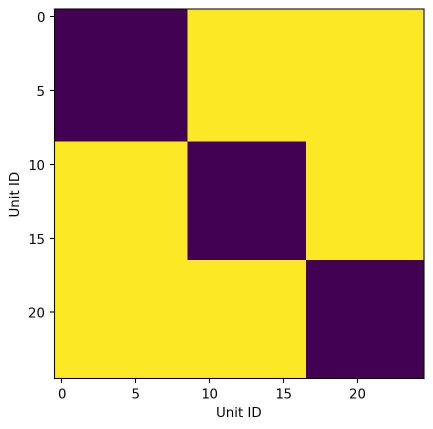
With data loaded in UnitMatch’s format, we can extract waveform parameters. The extract_parameter function takes as arguments the waveforms and channel positions, as well as a new dictionary clus_info, and returns a dictionary of extracted_wave_properties. ::: {.callout-warning} extract_parameters calculates the spatial decay by fitting an exponential function. In some cases (probably due to noisy data) the algorithm does not converge after the default number of iterations and throws an error. Unfortunately, there is no way to change the number of iteration other than editing the source code. There is an active GitHub issue on this - let’s hope it gets addressed soon. :::
clus_info = {
    "good_units": good_units,
    "session_switch": session_switch,
    "session_id": session_id,
    "original_ids": np.concatenate(good_units),
}
extracted_wave_properties = um.overlord.extract_parameters(
    waveform, channel_pos, clus_info, param
)
Let’s visualize two of those properties: the site where maximum amplitude was recorded for a given unit, and the coefficient with which the amplitude of that unit decays as we move away from that site. If these properties allow us to match units across sessions, we should start to see some clusters. The points for the 1st and 2nd half of a recording should be close together and we should see triplets that represent the same unit across all three sessions. Some clusters clearly contain more units, but that is to be expected since we only plotted 2 out of the 10 extracted waveform properties.
fig, ax = plt.subplots()
for i in range(2):
    ax.scatter(
        extracted_wave_properties["spatial_decay"][:, i],
        extracted_wave_properties["max_site"][:, i],
    )
ax.legend(labels=["1st Half", "2nd Half"])
ax.set(xlabel="Spatial Decay")
ax.set(ylabel="Maximum Site")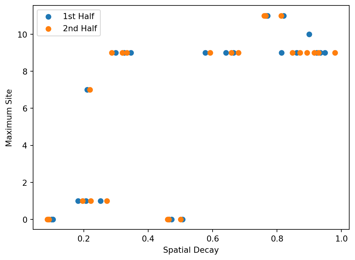
UnitMatch computes a total similarity score T (0-1) combining similarity across all waveform properties for each unit pair. The extract_metric_scores returns a matrix of total_score values and an array of candidate_pairs that marks all units where the match score exceeds the threshold. This threshold is determined automatically based on the similarity of the waveforms within each recording.
total_score, candidate_pairs, scores_to_include, predictors = (
    um.overlord.extract_metric_scores(
        extracted_wave_properties, session_switch, within_session, param, niter=2
    )
)
fig, ax = plt.subplots()
im = ax.imshow(total_score)
ax.contour(candidate_pairs, levels=[0.5], colors="red", linewidths=1.5)
ax.set(xlabel="Unit ID", ylabel="Unit ID")
cbar = plt.colorbar(im)
cbar.set_label("T")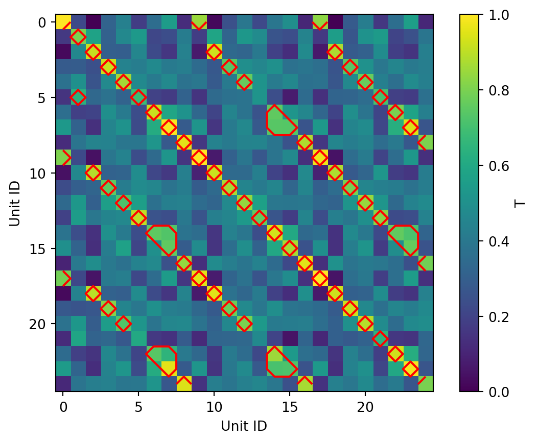
We now compute the prior probability that a random pair of units is a match, based on the number of putative matches that exceed the similarity score threshold.
p_nomatch = 1 - (param["n_expected_matches"] / param["n_units"] ** 2)
priors = np.array((p_nomatch, 1 - p_nomatch))
print(f"Prior probabilities: \nP(no match): {priors[0]} \nP(match): {priors[1]}")
Prior probabilities:
P(no match): 0.8784
P(match): 0.12160000000000004Then we calculate the likelihood distributions of all features for matches and non-matches, i.e. P(feature | match) and P(feature | non-match). The get_parameter_kernels function returns a 3D array of shape (s, k, 2) where s is the score and k is the feature.
labels = candidate_pairs.astype(int)
cond = np.unique(labels)
score_vector = param["score_vector"]
parameter_kernels = um.bayes_functions.get_parameter_kernels(
    scores_to_include, labels, cond, param, add_one=1
)

fig, ax = plt.subplots()
ax.plot(score_vector, parameter_kernels[:, i, 0], label="Non-matches")
ax.plot(score_vector, parameter_kernels[:, i, 1], label="Matches")
plt.legend()
ax.set(xlabel="Spatial decay score", ylabel="Density")
Calculating the probability distributions of the metric scores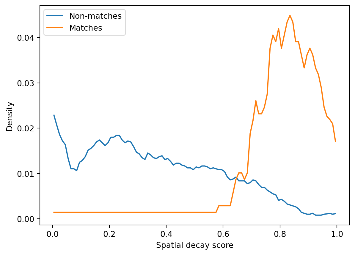
Finally, apply_naive_bayes multiplies feature likelihoods and applies Bayes’ theorem to compute the posterior probability that unit pairs match. The resulting probability matrix has the same shape as the similarity score matrix but its values are probabilities. We can select a probability threshold for units to be considered a match — here I use 0.9 but this is probably too strict for real data (in the original paper the authors use 0.5). Ideally, there should be three matches for every unit because it should match within each recording and across the other two recordings.
probability = um.bayes_functions.apply_naive_bayes(
    parameter_kernels, priors, predictors, param, cond
)
output_prob_matrix = probability[:, 1].reshape(param["n_units"], param["n_units"])
match_threshold = 0.9
output_threshold = np.zeros_like(output_prob_matrix)
output_threshold[output_prob_matrix > match_threshold] = 1
plt.imshow(output_threshold, cmap="Greys")
Calculating the match probabilities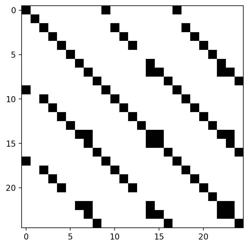
The matrix of matches above shows a clear pattern of bands that run parallel to the diagonal. This is because, in our simulation, units have the same order across recordings. This would not be the case for real recordings where you would see a more random, scattered pattern.
Combining Matches Across Recordings
While the probability matrix shows pairwise matching probabilities, our goal is tracking units across recordings. This is what the assign_unique_id function does — it groups units identified as matches across recordings while applying three different strategies: - Liberal: Groups units if they match with ANY unit in the proposed group. - Default: Groups units if they match with EVERY unit in adjacent sessions. - Conservative: Groups units only if they match with EVERY other unit in the proposed group.
In our case, the default and conservative strategies are almost identical since there are only 3 sessions, but for a larger number of sessions there should be a notable difference. We’ll proceed with the liberal strategy, although the original paper recommends using the conservative strategy.
matches = np.argwhere(output_threshold == 1)
UIDs = um.assign_unique_id.assign_unique_id(output_prob_matrix, param, clus_info)
unique_id = UIDs[0]  # liberal strategy
unique_id
Number of Liberal Matches: 26
Number of Intermediate Matches: 21
Number of Conservative Matches: 21array([ 0, 1, 2, 3, 4, 5, 6, 6, 8, 0, 2, 3, 4, 13, 6, 6, 8,
0, 2, 3, 4, 21, 6, 6, 8])Now, we combine all sortings using the aggregate_units function. Then, we identify matching units by identifying the locations of duplicates in the unique_id array. Finally, we use MergeUnitsSorting to merge and rename the units that have been matched. That’s it — now we have a sorting object that combines units across all sessions. The combined recording has 10 units despite only 8 surviving initial quality control. This shows that we were not able to find all existing matches (you can also see this from the missing squares in Figure 9).
sorting = aggregate_units(sortings)
units_to_merge = []
new_unit_ids = []
for uid in np.unique(unique_id):
    idx = np.where(unique_id == uid)[0]
    if len(idx) > 1:
        units_to_merge.append(list(sorting.unit_ids[idx]))
        new_unit_ids.append(uid)

sorting = MergeUnitsSorting(
    sorting, units_to_merge=units_to_merge, new_unit_ids=new_unit_ids
)
print(f"After merging there are {sorting.get_num_units()} units: \n{sorting.unit_ids}")
After merging there are 10 units:
['1' '5' '13' '21' '0' '2' '3' '4' '6' '8']UnitMatch also provides a save_to_output function that stores all of the estimated properties, distributions and probabilities. The cell below unpacks the extracted_wave_properties dictionary and saves the results to a folder called "out".
save_dir = "out"
amplitude = extracted_wave_properties["amplitude"]
spatial_decay = extracted_wave_properties["spatial_decay"]
avg_centroid = extracted_wave_properties["avg_centroid"]
avg_waveform = extracted_wave_properties["avg_waveform"]
avg_waveform_per_tp = extracted_wave_properties["avg_waveform_per_tp"]
wave_idx = extracted_wave_properties["good_wave_idxs"]
max_site = extracted_wave_properties["max_site"]
max_site_mean = extracted_wave_properties["max_site_mean"]
um.save_utils.save_to_output(
    save_dir,
    scores_to_include,
    matches,
    output_prob_matrix,
    avg_centroid,
    avg_waveform,
    avg_waveform_per_tp,
    max_site,
    total_score,
    output_threshold,
    clus_info,
    param,
    UIDs=UIDs,
    save_match_table=True,
)