Motivation⌗

The multivariate Temporal Response Function (mTRF) is widely used tool for modeling brain responses to continuous speech. The most popular package for using these models is the mTRF-Toolbox written in Matlab. We wrote mTRFpy to create an implementation that is open source and improves upon the intuitive and simple design of the original Matlab toolbox. Because researchers from various medical sub-fields (e.g. Psychiatry, Pediatrics) are increasingly interested in mTRF methods, we also provided extensive online tutorials that explain the technical details.

Design⌗

The original mTRF-Toolbox was a set of functions. We instead used an object oriented design that allows the user to perform most mTRF analyses by interacting with only the TRF class. This class stores all important properties such as the models sampling rate, time points and model weights associated with different features.

Because we wanted to make the transition for users of the original toolbox easy and intuitive, we used similar naming patters for our class methods (e.g. the method TRF.train() in mTRFpy corresponds the function mTRFtrain() in the original toolbox). We also use an automated testing pipeline to ensure that mTRFpy and the mTRF-Toolbox produce the same result for the same analysis ¹.

In addition to the TRF class, mTRFpy also provides a stats module that implements functions for statistical inference that were not part of the original mTRF-toolbox. These functions include nested cross-validation and permutation which allows the user to compute unbiased estimates of model accuracy and test their significance ².

To keep the toolbox light with a minimal number of dependencies, we implemented everything in pure Python and Numpy. This makes mTRFpy easily compatible with most existing analysis pipelines and leverages potential synergies with the Python machine learning ecosystem.

Example⌗

In the blow example, we are computing a model which predicts one persons EEG responses as they were listening to an audiobook based on a 16-band spectrogram of said audiobook. This data is provided by mTRFpy and can be obtained via the function load_sample_data, which also segments and normalizes the data.

Then, we define the range of time lags across which the model is computed and define a list of regularization coefficients ³. Those variables are passed to the TRF.train() method which tests all candidate regularization values and finds the one that yields the most accurate model.

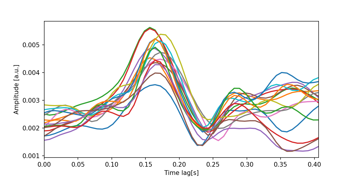
Finally, we visualize the optimized model by computing the global field power (i.e. the standard deviation across all recorded EEG channels) for each spectral band.

from mtrf import TRF, load_sample_data

stimulus, response, fs = load_sample_data(n_segments=10, normalize=True)
tmin, tmax = 0, 0.4
regularization = [0.1, 1, 10, 100, 1000, 10000, 100000]

trf = TRF()
r = trf.train(stimulus, response, fs, tmin, tmax, regularization)

print(f'Best model: regularization={trf.regularization}, r={r.max().round(3)}')
trf.plot(channel='gfp')

The below plot can be interpreted as the expected change in the neural response following a change in the predictor. For example, the peaks indicate that there is an increase in the neural response roughly 150 milliseconds after there was an increase in spectral power in the respective bands.

Resources⌗

You can install mTRFpy from PyPI via pip install mtrf. You can find extensive tutorials on the project’s website and view the source code on GitHub. A corresponding paper can be found in the Journal of Open Source science.

Footnotes⌗